Commandline Capture of HDF Files Tutorial#
This tutorial shows how to use the commandline tool to save an HDF file from the PandA
for each PCAP acquisition. It assumes that you have followed the tutorial-load-save tutorial
to setup the PandA.
Capturing some data#
In one terminal launch the HDF writer client, and tell it to capture 3 frames in a location of your choosing:
pandablocks hdf <hostname> --num=3 /tmp/panda-capture-%d.h5
Where <hostname> is the hostname or ip address of your PandA. This will connect
to the data port of the PandA and start listening for up to 3 acquisitions. It will
then write these into files:
/tmp/panda-capture-1.h5
/tmp/panda-capture-2.h5
/tmp/panda-capture-3.h5
In a second terminal you can launch the acquisition:
$ pandablocks control <hostname>
< *PCAP.ARM=
OK
This should write 1000 frames at 500Hz, printing in the first terminal window:
INFO:Opened '/tmp/panda-capture-1.h5' with 60 byte samples stored in 11 datasets
INFO:Closed '/tmp/panda-capture-1.h5' after writing 1000 samples. End reason is 'Ok'
You can then do PCAP.ARM= twice more to make the other files.
Examining the data#
You can use your favourite HDF reader to examine the data. It is written in swmr
mode so that you can read partial acquisitions before they are complete.
Note
Reading SWMR HDF5 files while they are being written to require the use of a Posix compliant filesystem like a local disk or GPFS native client. NFS mounts are not Posix compliant.
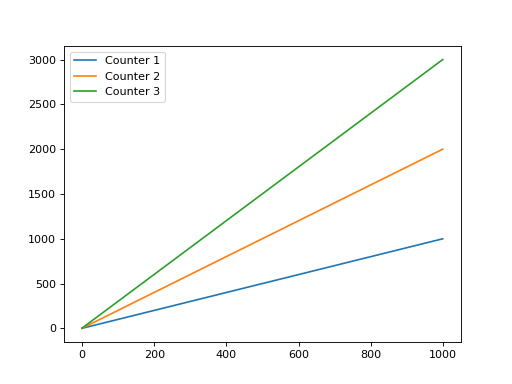
In the repository examples/plot_counter_hdf.py is an example of reading the
file, listing the datasets, and plotting the counters:
import sys

import h5py
import matplotlib.pyplot as plt

if __name__ == "__main__":
    with h5py.File(sys.argv[1], "r") as hdf:
        # Print the dataset names in the file
        datasets = list(hdf)
        print(datasets)
        # Plot the counter mean values for the 3 counters we know are captured
        for i in range(1, 4):
            plt.plot(hdf[f"COUNTER{i}.OUT.Mean"], label=f"Counter {i}")
        # Add a legend and show the plot
        plt.legend()
        plt.show()
Running it on /tmp/panda-capture-1.h5 will show the three counter values:
(Source code, png, hires.png, pdf)

You should see that they are all the same size:
$ ls -s --si /tmp/panda-capture-*.h5
74k /tmp/panda-capture-1.h5
74k /tmp/panda-capture-2.h5
74k /tmp/panda-capture-3.h5
If you have h5diff you can check the contents are the same:
$ h5diff /tmp/panda-capture-1.h5 /tmp/panda-capture-2.h5
$ h5diff /tmp/panda-capture-1.h5 /tmp/panda-capture-3.h5
Absolute timestamps#
Starting with v3.0, PandABox firmware supports absolute timestamping of the collected data. PandA still collects relative timestamps for individual data points that are saved as arrays to HDF5 file. In addition, the absolute timestamp for the start of the measurement is saved to HDF5 file and can be used to convert relative timestamps to absolute timestamps
The absolute timestamp is saved as a set of attributes of the root group of the HDF5 file. The attributes are optional and set only if the respective parameters were captured by PandABox and received by the IOC. The following attributes are used:
arm_time- the time when the Panda (PCAP block) was armed, saved as a string in the ISO 8601 UTC format. This parameter is mostly used for debugging.start_time- the start time (PCAP block is armed and enabled) of the measurement in seconds since the epoch, saved as a string in the ISO 8601 UTC format. Uses hardware provided timestamp (e.g. PTP or MRF) if available, falling back to the system timestamp.hw_time_offset_ns- the offset in nanoseconds (int64) that should be added to tostart_timeto get back to the system timestamp. The attribute is present only if Panda is configured to use hardware-based absolute timestamps (PTP or MRF).
The following code may be used to read the absolute timestamp from the HDF5 file.
Use pandas.Timestamp object if nanosecond accuracy is required (standard
dataframe object is limited to microsecond precision).
import sys

import h5py
import pandas as pd

if __name__ == "__main__":
    with h5py.File(sys.argv[1], "r") as f:
        arm_time = f.attrs.get("arm_time", None)
        start_time = f.attrs.get("start_time", None)
        hw_time_offset_ns = f.attrs.get("hw_time_offset_ns", None)

        print(f"Arm time: {arm_time!r}")
        print(f"Start time: {start_time!r}")
        print(f"Hardware time offset: {hw_time_offset_ns!r} ns")

        if start_time:
            # Compute and print the start time that includes the offset
            ts_start = pd.Timestamp(start_time)
            if hw_time_offset_ns:
                ts_start += pd.Timedelta(nanoseconds=hw_time_offset_ns)
            print(f"Start time (system clock instead of hardware clock): {ts_start}")


# Expected output:
#
# Arm time: '2024-03-05T20:27:12.607841574Z'
# Start time: '2024-03-05T20:27:12.605729480Z'
# Hardware time offset: 2155797 ns
# Start TS including the offset: 2024-03-05T20:27:08.605729480Z
Collecting more data faster#
The test data is produced by a SEQ Block, configured to produce a high level for 1 prescaled tick, then a low level for 1 prescaled tick. The default setting is to produce 1000 repeats of these, with a prescale of 1ms and hence a period of 2ms. Each sample is 11 fields, totalling 60 bytes, which means that it will produce data at a modest 30kBytes/s for a total of 2s. We can increase this to a more taxing 30MBytes/s by reducing the prescaler to 1us. If we increase the prescaler to 10 million then we will sustain this data rate for 20s and write 600MByte files each time:
$ pandablocks control <hostname>
< SEQ1.REPEATS?
OK =1000  # It was doing 1k samples, change to 10M
< SEQ1.REPEATS=10000000
OK
< SEQ1.PRESCALE?
OK =1000
< SEQ1.PRESCALE.UNITS?
OK =us  # It was doing 1ms ticks, change to 1us
< SEQ1.PRESCALE=1
OK
Lets write a single file this time, telling the command to also arm the PandA:
pandablocks hdf <hostname> --arm /tmp/biggerfile-%d.h5
Twenty seconds later we will get a file:
$ ls -s --si /tmp/biggerfile-*.h5
602M /tmp/biggerfile-1.h5
Which looks very similar when plotted with the code above, just a bit bigger:
(Source code, png, hires.png, pdf)

Conclusion#
This tutorial has shown how to capture data to an HDF file using the commandline
client. It is possible to use this commandline interface in production, but it is
more likely to be integrated in an application that controls the acquisition as well
as writing the data. This is covered in library-hdf. You can explore strategies
on getting the maximum performance out of a PandA in performance.